


1. Introduction
The past few years have seen a growing interest in understanding of pressure-driven channel flows of dilute polymer solutions (Castillo Sánchez et al. Reference Castillo Sánchez, Jovanović, Kumar, Morozov, Shankar, Subramanian and Wilson2022; Datta et al. Reference Datta2022). The state space of such flows is spanned by three dimensionless parameters:  $Re$, the Reynolds number that measures the relative importance of inertia compared with viscous dissipation;
  ${{Wi}}$, the Weissenberg number that measures the strength of polymer-induced viscoelastic stresses;
  $\beta$, the solvent to the total solution viscosity ratio that is related to the polymer concentration. The rich variety of flow states associated with different parts of the
  $(Re,{{Wi}},\beta )$ space ranges from drag-reduction and elasto-inertial turbulence (Dubief, Terrapon & Hof Reference Dubief, Terrapon and Hof2023) to purely elastic instabilities and turbulence (Steinberg Reference Steinberg2021), making it a subject of interest for turbulence and flow-control researchers, polymer rheologists and physicists studying flows of complex fluids (Castillo Sánchez et al. Reference Castillo Sánchez, Jovanović, Kumar, Morozov, Shankar, Subramanian and Wilson2022; Datta et al. Reference Datta2022).
The most significant recent advances in this area correspond to flows with small to negligible amounts of inertia. Such flows were believed to be laminar and exhibit no instabilities, until several studies challenged this view. While early results on pressure-driven channel flows of model dilute polymer solutions indicated their linear stability (Gorodtsov & Leonov Reference Gorodtsov and Leonov1967; Wilson, Renardy & Renardy Reference Wilson, Renardy and Renardy1999), Morozov & van Saarloos (Reference Morozov and van Saarloos2005, Reference Morozov and van Saarloos2007, Reference Morozov and van Saarloos2019) proposed a subcritical bifurcation from infinity as a nonlinear destabilisation mechanism, similar to Newtonian wall-bounded shear flows (Eckhardt Reference Eckhardt2018; Graham & Floryan Reference Graham and Floryan2021). The existence of such a subcritical bifurcation was demonstrated experimentally by Arratia and co-workers (Pan et al. Reference Pan, Morozov, Wagner and Arratia2013; Qin & Arratia Reference Qin and Arratia2017; Qin et al. Reference Qin, Salipante, Hudson and Arratia2019), while the more recent experiments by Steinberg and co-workers (Jha & Steinberg Reference Jha and Steinberg2020, Reference Jha and Steinberg2021; Shnapp & Steinberg Reference Shnapp and Steinberg2022; Li & Steinberg Reference Li and Steinberg2022) provide insight into the spatial structure of the ensuing instability.
In addition to these developments, Shankar and co-workers re-visited the linear stability analysis of pressure-driven channel flows of model dilute polymer solutions, and identified a novel linear instability mechanism associated with the centre-line mode (Chaudhary et al. Reference Chaudhary, Garg, Shankar and Subramanian2019; Khalid, Shankar & Subramanian Reference Khalid, Shankar and Subramanian2021b; Khalid et al. Reference Khalid, Chaudhary, Garg, Shankar and Subramanian2021a). Although this linear instability exists in a narrow range of parameters,  $1-\beta \ll 1$ and
  ${{Wi}}\gg 1$, which can be difficult to simultaneously realise experimentally, the nonlinear structures that stem from this instability appear to be crucial to the understanding of elasto-inertial and purely elastic channel flows. Page, Dubief & Kerswell (Reference Page, Dubief and Kerswell2020) and Buza, Page & Kerswell (Reference Buza, Page and Kerswell2022) showed that for sufficiently large values of
  $Re$, the linear instability discussed above leads to a two-dimensional subcritical bifurcation that extends significantly outside of the
  $(Re,{{Wi}})$ region where the linear instability exists. Morozov (Reference Morozov2022) performed direct numerical simulations of two-dimensional channel flow at negligible inertia,
  $Re\ll 1$, for a wide range of
  $\beta$ and
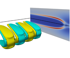
  ${{Wi}}$, and reported the existence of purely elastic nonlinear travelling-wave solutions. These solutions, that we will refer to as the narwhals, appear through a bifurcation from infinity that ties their existence with the original proposal by Morozov & van Saarloos (Reference Morozov and van Saarloos2005, Reference Morozov and van Saarloos2007, Reference Morozov and van Saarloos2019). (Previous work referred to similar structures as arrowheads (Page et al. Reference Page, Dubief and Kerswell2020; Buza et al. Reference Buza, Page and Kerswell2022; Dubief et al. Reference Dubief, Page, Kerswell, Terrapon and Steinberg2022). We do not appreciate the association of that term with warfare, and, instead, prefer to call them narwhals, for the obvious likeness of their polymer stress distribution (see figure 1, for example). We are grateful to Professor Becca Thomases (Smith College) for suggesting the name.) Their obvious centre-mode character and their visual resemblance to the structures reported in the elasto-inertial regime (Page et al. Reference Page, Dubief and Kerswell2020; Buza et al. Reference Buza, Page and Kerswell2022; Dubief et al. Reference Dubief, Page, Kerswell, Terrapon and Steinberg2022) most likely imply that these structures belong to the same solution family that is ultimately connected to the centre-mode linear instability found in a rather special part of the
  $(\beta,{{Wi}},Re)$ parameter space.

Figure 1. Examples of two-dimensional narwhal travelling-wave solutions used as the base state in our linear stability analysis. (a) A purely elastic state with  $({{Wi}}, \beta, Re)$ =
  $(100, 0.8, 0.01)$ and
  $L_x=10$, studied in Morozov (Reference Morozov2022). (b) An elasto-inertial state with
  $({{Wi}}, \beta, Re)$ =
  $(45, 0.997, 90)$ and
  $L_x = 2{\rm \pi} /2.18$, motivated by the work of Page et al. (Reference Page, Dubief and Kerswell2020). (c) A purely elastic state connected to the centre-mode instability found by Khalid et al. (Reference Khalid, Shankar and Subramanian2021b) with
  $({{Wi}}, \beta, Re) = (1700, 0.997, 0.01)$ and
  $L_x = 2{\rm \pi} /0.75$. The colours indicate values of
  ${\rm tr}(\boldsymbol {c})$ and solid lines show the streamlines of the velocity deviation from the streamwise-averaged flow profile. The mean flow is from left to right along the
  $x$-direction.
While the narwhal solutions share many of the features observed in experiments (Pan et al. Reference Pan, Morozov, Wagner and Arratia2013; Qin & Arratia Reference Qin and Arratia2017; Qin et al. Reference Qin, Salipante, Hudson and Arratia2019; Jha & Steinberg Reference Jha and Steinberg2020, Reference Jha and Steinberg2021; Shnapp & Steinberg Reference Shnapp and Steinberg2022; Li & Steinberg Reference Li and Steinberg2022), they do not represent chaotic flows; indeed, in two-dimensional channel flows, they are steady travelling-wave solutions. To be dynamically relevant, these structures are expected to lose their stability when embedded in three-dimensional domains, as is indeed the case with Newtonian Tollmien–Schlichting waves (Orszag & Patera Reference Orszag and Patera1983). The purpose of the current work is to study the three-dimensional linear stability of the two-dimensional narwhal solutions discussed above. We report that in all cases studied here for a wide range of  $\beta$,
  ${{Wi}}$ and
  $Re$, the two-dimensional narwhal solutions lose their stability when embedded in a three-dimensional domain. We characterise this instability and discuss its implications for the mechanism of elastic and elasto-inertial turbulence.
2. Equations of motion and numerical details
We consider three-dimensional pressure-driven channel flow and select a Cartesian coordinate system with  $(x,y,z)$ being along the flow (streamwise), wall-normal and spanwise directions, correspondingly. The dimensionless equations of motion for the polymeric fluid are given by the Phan-Thien–Tanner (PTT) constitutive model (Phan-Thien & Tanner Reference Phan-Thien and Tanner1977), coupled to the incompressible Navier–Stokes equation:
 \begin{gather} \partial_t \boldsymbol{c}+\boldsymbol{u}\boldsymbol{\cdot}\boldsymbol{\nabla}\boldsymbol{c}-\boldsymbol{\nabla} \boldsymbol{u}^{\dagger}\boldsymbol{\cdot}\boldsymbol{c}-\boldsymbol{c}\boldsymbol{\cdot}\boldsymbol{\nabla} \boldsymbol{u} ={-}\frac{\boldsymbol{c}-\boldsymbol{1}}{{{Wi}}}(1-3\epsilon+\epsilon~ {\rm tr}(\boldsymbol{c})) + \kappa \Delta \boldsymbol{c}, \end{gather}
 \begin{gather}\partial_t \boldsymbol{u} + \boldsymbol{u}\boldsymbol{\cdot}\boldsymbol{\nabla} \boldsymbol{u} ={-}\boldsymbol{\nabla}p + \frac{\beta}{Re}\Delta \boldsymbol{u} + \frac{1-\beta}{Re {{Wi}}} \boldsymbol{\nabla}\boldsymbol{\cdot} \boldsymbol{c}+\frac{2}{Re}\boldsymbol{e}_x, \end{gather}
 \begin{gather}\boldsymbol{\nabla}\boldsymbol{\cdot}\boldsymbol{u} = 0 , \end{gather}
where the dagger denotes the transpose,  $\boldsymbol {1}$ is the identity matrix,
  ${\rm tr}$ denotes the trace,
  $\boldsymbol {e}_x$ is the unit vector in the
  $x$-direction,
  $\boldsymbol {u}$ is the fluid velocity,
  $\boldsymbol {c}$ is the polymer conformation tensor and
  $p$ is the pressure. The equations are rendered dimensionless by using
  $d$,
$d$,  $\mathcal {U}$,
  $d/\mathcal {U}$,
  $\eta _p \mathcal {U} / d$ and
  $(\eta _s+\eta _p)\mathcal {U}/d$ as the scales for length, velocity, time, stress and pressure, respectively. Here,
  $d$ is the channel half-width,
  $\eta _s$ and
  $\eta _p$ are the solvent and polymeric contributions to the viscosity, and
  $\mathcal {U}$ is the centre-line value of the laminar fluid velocity of a Newtonian fluid with the viscosity
  $\eta _s+\eta _p$ at the same value of the applied pressure gradient. As discussed above, the state diagram of this flow is spanned by the viscosity ratio
  $\beta =\eta _s/(\eta _s+\eta _p)$, the Reynolds number
  $Re=\rho \mathcal {U} d/(\eta _s+\eta _p)$ and the Weissenberg number
  ${{Wi}}= \lambda \mathcal {U} / d$, where
  $\rho$ is the density of the fluid and
  $\lambda$ is the Maxwell relaxation time of polymer molecules. Finally, the constant
  $\epsilon$ controls the degree of shear-thinning of the model PTT fluid, and
  $\kappa$ is a dimensionless polymer diffusivity. The stress-diffusion term in (2.1) is added to ensure that the conformation tensor
  $\boldsymbol {c}$ remains strictly positive-definite at all times throughout our work. We note that while some previous studies employed unrealistically large values of
  $\kappa$ for this purpose, the value of
  $\kappa$ used here is in line with the realistic values relevant to microfluidic experiments (Pan et al. Reference Pan, Morozov, Wagner and Arratia2013; Qin & Arratia Reference Qin and Arratia2017; Qin et al. Reference Qin, Salipante, Hudson and Arratia2019). See Morozov (Reference Morozov2022) for the estimates of
  $\kappa$ and its relationship to kinetic theories of dilute polymer solutions.
The starting point of our analysis are the narwhal travelling-wave solutions determined in Morozov (Reference Morozov2022) by numerically advancing the two-dimensional version of (2.1)–(2.3) in time until a steady state was reached. We denote those states by  $s_{2D}=\{\boldsymbol {u}_{2D}, p_{2D}, \boldsymbol {c}_{2D}\}(x-\phi _{2D} t, y)$, where
  $\phi _{2D}$ is the phase speed of the travelling wave. For each narwhal state, the corresponding value of
  $\phi _{2D}$ was determined numerically by tracking the spatial position of the largest value of
  ${\rm tr}(\boldsymbol {c}_{2D})$ as a function of time. In what follows,
  $s_{2D}$ and
  $\phi _{2D}$ serve as the base state for our linear stability calculations.
To probe the linear stability of the two-dimensional narwhal states  $s_{2D}$ with respect to three-dimensional infinitesimal perturbations in the form
  $s_{3D}=\{\delta \boldsymbol {u}, \delta p, \delta \boldsymbol {c}\}(x-\phi _{2D} t, y, z, t)$, we linearise (2.1)–(2.3) in three dimensions around a two-dimensional travelling-wave state
  $s_{2D}=\{\boldsymbol {u}_{2D}, p_{2D}, \boldsymbol {c}_{2D}\}(x-\phi _{2D} t, y)$. The resulting linear equations for
  $s_{3D}$ are stepped forward in time to determine the growth rate of the instability. The methodology employed here is similar to that used by Orszag & Patera (Reference Orszag and Patera1983), who studied stability of Newtonian Tollmien–Schlichting waves. As the linearised equations of motion for
  $s_{3D}$ decouple the time evolution of the Fourier modes in the
  $z$-direction, the full dispersion relation can be obtained from a single three-dimensional simulation. To this end, we introduce an observable
  $a(t,k_z)$ that is based on
  $s_{3D}$ as follows:
 \begin{equation} a(t, k_z) =\left\langle\hat{\delta c}_{xx}(x-\phi_{2D} t, y, k_z, t) \hat{\delta c}_{xx}^*(x-\phi_{2D} t, y, k_z, t)\right\rangle_{x,y}. \end{equation}
Here, the hat denotes the Fourier transform along the  $z$-direction,
  $k_z$ is the wave number, and
  $\langle \cdots \rangle _{x,y}$ denote spatial average over the
  $x$- and
  $y$-directions. While
  $a(t,k_z)$ can, in principle, be defined based on any component of
  $s_{3D}$, here we singled out
  $\delta c_{xx}$ as it is the largest component of the conformation tensor and is the most dynamically active one. As we will see below, for sufficiently long times,
  $a(t,k_z)\sim e^{2 \sigma (k_z) t}$, with
  $\sigma (k_z)$ being the real part of the leading eigenvalue. All eigenvalues reported in this work have zero imaginary parts up to numerical accuracy. Below, we refer to
  $\sigma =\sigma (k_z)$ as the dispersion relation.
Simulations are carried out using a parallel pseudo-spectral solver with full  $3/2$-dealiasing implemented in Dedalus (Burns et al. Reference Burns, Vasil, Oishi, Lecoanet and Brown2020) on a domain
  $[0, L_x]\times [-1, 1]\times [0, L_z]$, where
  $L_x$ and
  $L_z$ are the dimensionless system size in the streamwise and spanwise directions, respectively. We employ no-slip boundary conditions for the velocity,
  $\delta \boldsymbol {u}(x-\phi _{2D} t, y=\pm 1, z, t)=0$, and natural boundary conditions for the conformational stress tensor, where
  $\delta \boldsymbol {c}(x-\phi _{2D} t, y=\pm 1, z, t)$ is set to the corresponding values of (2.1) with
  $\kappa =0$ at each time step (Liu & Khomami Reference Liu and Khomami2013); periodic boundary conditions are used in the streamwise and spanwise directions. All fields are represented by Fourier decompositions in the periodic directions, and by a Chebyshev expansion in the
  $y$-direction using
  $N_x \times N_y \times N_z = 256 \times 1024 \times 128$ spectral modes. The time stepping uses a four-stage, third-order implicit-explicit Runge–Kutta method with the time step
  $dt=5\times 10^{-3}$. Each simulation is started from an
  $s_{2D}$ narwhal state. To break its translational invariance in the
  $z$-direction, the perturbation component
  $\delta c_{xx}$ is initialised with a Gaussian noise of zero mean and unit variance; the magnitude of the noise is selected to be
  $1\times 10^{-7}$ of the maximum value of the
  $c_{xx}$ component of the narwhal conformation tensor.
3. Results
First, we analyse linear stability of the purely elastic narwhal solutions reported in Morozov (Reference Morozov2022); see figure 1(a), for example. We set  $L_x=L_z=10$,
  $Re=0.01$,
  $\epsilon = 10^{-3}$,
  $\kappa = 5\times 10^{-5}$ and vary
  $\beta$ and
  ${{Wi}}$. For these parameters, the laminar flow is linearly stable, and the two-dimensional travelling-wave solutions appear through a subcritical bifurcation from infinity. In what follows, the lowest value of
  ${{Wi}}$ for each
  $\beta$ considered here corresponds to the saddle-node of the subcritical bifurcation.
In figure 2(a), we present a typical evolution of the observable  $a(t,k_z)$ for various values of
  $k_z$. As our initial condition comprises Gaussian noise, the initial projection on the most unstable eigenmode is small, and
  $a(t,k_z)$ initially decreases as a function of time. At sufficiently long times, the time evolution of
  $a(t,k_z)$ is dominated by the largest unstable eigenvalue that we determine by fitting an exponential
  $a(t,k_z)\sim e^{2\sigma (k_z) t}$ to its long-
 $t$ behaviour, as discussed above. Examples of such fits are given by the dashed lines in figure 2(a). Combining
  $\sigma (k_z)$ as a function of
  $k_z$ yields the dispersion relation for given
  $\beta$ and
  ${{Wi}}$, and, in figure 2(b), we show several representative examples. All dispersion relations studied in this work have the same shape, and exhibit a peak in the
  $\sigma (k_z)$ curves, indicating an instability with a finite spanwise length scale. The largest growth rates and the corresponding values of
  $k_z$ are presented in figure 3. We conclude that all two-dimensional narwhal solutions become linearly unstable when embedded in a three-dimensional domain.

Figure 2. (a) Time evolution of the observable  $a(t, k_z)$ defined in (2.4) for
  $({{Wi}}, \beta ) = (100, 0.7)$ and selected wave numbers. The black dashed lines show the exponential fits used to measure the growth rate
  $\sigma (k_z)$. (b) Dispersion relations for representative example values of
  $({{Wi}}, \beta )$. The symbols superposed on the
  $({{Wi}}, \beta ) = (100, 0.7)$ data (orange curve) represent the values of the growth rates determined from (a).

Figure 3. Results of linear stability analysis for the purely elastic narwhal solutions found in Morozov (Reference Morozov2022). (a) The growth rates of the most unstable mode,  $\sigma _{max} = \max _{k_z} \sigma (k_z)$, for various
  $\beta$ and
  ${{Wi}}$. (b) The corresponding values of
  $k_z$ that set the spanwise periodicity of the most unstable mode.
To gain insight into the spatial structure of the instability, in figure 4 we plot the three-dimensional profile associated with the most unstable mode (the peak of  $\sigma (k_z)$) for
  $\beta =0.8$ and
  ${{Wi}}=100$. For clarity, we only report a part of the simulation domain that contains a few instability periods in the spanwise direction, set by
  $k_{z,max}^{-1}$. As can be seen from figure 4(a,c), the polymer extension associated with the perturbation,
  ${\rm tr}(\delta \boldsymbol {c})$, is localised in thin sheets around the polymer extension of the base flow (the ‘body’ of the narwhal), with regions of polymer stretch and compression alternating along the spanwise direction. This stress distribution drives a periodic array of vortices that are primarily confined to the streamwise-spanwise centre-plane, with the maxima/minima of the streamwise component of the velocity perturbation coinciding with the stretching/compression of the polymers.

Figure 4. Representative example of the three-dimensional spatial profiles of the most unstable mode for  $({{Wi}}, \beta ) = (100, 0.8)$ with
  $k_z\approx 6.91$. The two-dimensional base narwhal state is shown in the background of all subfigures, with the colour scheme indicating the magnitude of
  ${\rm tr}(\boldsymbol {c}_{2D})$. For visualisation purposes we show either one or two periods of the perturbation in the spanwise direction only. (a) Isosurfaces of the perturbation
  ${\rm tr}(\delta \boldsymbol {c})$, with light/dark colour showing polymer extension/compression. The same structures are shown in (b) alongside the perturbation velocity field, shown by the arrows, and the centre-plane streamfunction, shown by the solid lines. (c) Planar view of the base state and a half-period of the perturbation that demonstrates that the perturbation stresses are localised on both sides of the narwhal ‘body’, as discussed in the main text.
Up to this point, our analysis was restricted to the case of the subcritical travelling-wave solutions that are disconnected from the laminar state. Next, we consider two sets of parameter values where the narwhal solutions are known to connect to a two-dimensional linear instability of the base state. The first corresponds to the purely elastic instability identified for  $1-\beta \ll 1$ and
  ${{Wi}}\ll 1$ by Khalid et al. (Reference Khalid, Shankar and Subramanian2021b). To match the parameters of the linear instability identified in that work, we set
  $L_x=2{\rm \pi} /0.75$,
  $L_z=10$,
  $Re=0.01$,
  ${{Wi}}=1700$ and
  $\beta = 0.997$. To demonstrate that the three-dimensional instability reported here also exists in the elasto-inertial regime, we consider the following set of parameters motivated by the work of Page et al. (Reference Page, Dubief and Kerswell2020):
  $L_x=2{\rm \pi} /2.18$,
  $L_z=10$,
  $Re=90$,
  ${{Wi}}=45$ and
  $\beta = 0.9$. In both cases we set
  $\epsilon = 5\times 10^{-5}$ and
  $\kappa = 3\times 10^{-5}$.
For these two sets of parameters, we performed two-dimensional direct numerical simulations, similar to Morozov (Reference Morozov2022), and obtained steady travelling-wave solutions, shown in figure 1. Note that our elasto-inertial narwhal solution differs slightly from that obtained by Page et al. (Reference Page, Dubief and Kerswell2020), as those authors considered constant-flux channel flow, while we study the constant-pressure-gradient case. In figure 5, we present the dispersion relation of the three-dimensional linear stability analysis for these two sets of parameters. Although the high- ${{Wi}}$, high-
 $\beta$ case associated with the centre-mode instability in two dimensions leads to a significantly weaker three-dimensional instability, yet again, both two-dimensional structures are linearly unstable when embedded in three-dimensional domains.

Figure 5. Dispersion relations for  $({{Wi}}, \beta, Re) = (1700,0.997,0.01)$ and
  $(L_x, L_z) = (2{\rm \pi} /0.75, 10)$ (open squares), and
  $({{Wi}}, \beta, Re) = (45,0.9,90)$ and
  $(L_x, L_z) = (2{\rm \pi} /2.18, 10)$ (open circles).
4. Discussion
Recent numerical studies of pressure-driven channel flows of dilute polymer solutions identified narwhal travelling-wave solutions as steady coherent structures dominating purely elastic (Buza et al. Reference Buza, Page and Kerswell2022; Morozov Reference Morozov2022) and elasto-inertial (Page et al. Reference Page, Dubief and Kerswell2020; Dubief et al. Reference Dubief, Page, Kerswell, Terrapon and Steinberg2022) two-dimensional flows. In this work, we analysed linear stability of these two-dimensional structures upon their embedding in three-dimensional domains. In all parts of the parameter space  $(Re,{{Wi}},\beta )$ studied here, both purely elastic and elasto-inertial, we find that the narwhal solutions become linearly unstable to perturbations periodic in the spanwise direction. The structure of the unstable mode and the shape of the dispersion relation are reminiscent of the linear instability reported in the literature in viscoelastic flows with strong spatial gradients of the polymer normal stress (Renardy Reference Renardy1988; Hinch et al. Reference Hinch1992) and in shear-banded flows (Fielding & Wilson Reference Fielding and Wilson2010; Nicolas & Morozov Reference Nicolas and Morozov2012). Here, the role of the surface of large polymer extension is played by the thin sheets of high polymer stress constituting the body of the narwhal solution, as can be seen from figure 1. This observation is supported by figure 4(c) that shows that the polymer stretch associated with the three-dimensional perturbation is confined to a narrow vicinity of the high-stress region of the narwhal base state. While the instability exists for a wide range of the wave numbers
  $k_z$, the length scale associated with the most unstable mode, figure 3(b), is commensurate with the extent of the narwhal body in the wall-normal direction. As can also be seen from figure 3(a), the instability time scale is sufficiently short to result in a quick transition away from the base two-dimensional state.
Stability properties of the narwhal solutions reported above mirror closely the behaviour of Tollmien–Schlichting travelling-wave solutions in Newtonian pressure-driven channel flows. There, stable two-dimensional Tollmien–Schlichting waves appear through a linear instability at  $Re=5772$ in sufficiently long domains (Orszag Reference Orszag1971), and extend subcritically to significantly lower values of
  $Re$ (Herbert Reference Herbert1976). Infinitesimal three-dimensional perturbations are, however, sufficient to drive the flow away from the two-dimensional structures, leading directly towards the turbulent state (Orszag & Patera Reference Orszag and Patera1983). The analogy with the Tollmien–Schlichting waves has significant implications for our understanding of turbulent dynamics in the presence of polymers. Since the narwhal solutions are unstable in three dimensions, they can be seen as an effective route to ignite purely elastic or elasto-intertial turbulence. However, similar to Tollmien–Schlichting waves in the Newtonian case, narwhal solutions are unlikely to be dynamically relevant in three dimensions. There are two reasons for this. Firstly, the solutions are low-dimensional and will therefore only occupy a small region in the high-dimensional phase space of a three-dimensional chaotic flow. Secondly, as we show here, narwhal solutions are unstable to perturbations at many length scales, hence any phase-space trajectory is unlikely to spend sufficiently long time in their vicinity. While recent studies suggested that elasto-inertial turbulence could be quasi-two-dimensional in nature (Dubief, Terrapon & Soria Reference Dubief, Terrapon and Soria2013; Samanta et al. Reference Samanta, Dubief, Holzner, Schäfer, Morozov, Wagner and Hof2013; Sid, Terrapon & Dubief Reference Sid, Terrapon and Dubief2018; Shekar et al. Reference Shekar, McMullen, Wang, McKeon and Graham2019, Reference Shekar, McMullen, McKeon and Graham2021), our results demonstrate that no conclusions about purely elastic or elasto-inertial flows can be drawn from studying strictly two-dimensional versions of such flows; their properties can only be accessed by three-dimensional simulations.
Acknowledgements
We gratefully acknowledge the support we received from the Dedalus team (https://dedalus-project.org), and Keaton Burns in particular.
Funding
Computational resources on ARCHER2 (www.archer2.ac.uk) were provided by the UK Turbulence Consortium (https://www.ukturbulence.co.uk/, EPSRC grant number EP/R029326/1). We acknowledge financial support from the German Academic Scholarship Foundation (Studienstiftung des deutschen Volkes) and this work received funding from Priority Programme SPP 1881 ‘Turbulent Superstructures’ of the Deutsche Forschungsgemeinschaft (DFG, grant number Li3694/1). For the purpose of open access, the authors have applied a Creative Commons Attribution (CC BY) licence to any Author Accepted Manuscript version arising from this submission.
Declaration of interests
The authors report no conflict of interest.


 Open access